Atmospheric General Circulation Model
General circulation models (GCMs) are widely used for weather forecasting, seasonal prediction, and climate simulation. GCMs are conceptually divided into two components: a resolved dynamical fluid flow component; and an unresolved, sub-grid-scale component, which is parameterized as functions of the large-scale, resolved flow. We call the resolved component the dynamical core, and the parameterized component the physical parameterization. The atmospheric component model of CAS ESM (Chinese Academy of Sciences Earth System Model) is IAP AGCM (Institute of Atmospheric Physics Atmospheric General Circulation Model), which was first released in the 1980s. The latest version of the model is IAP AGCM4.1, which has a horizontal resolution of approximately 1.4° latitude × 1.4° longitude and 30 vertical levels. The dynamical core of IAP AGCM4.1 uses a finite-difference scheme based on a regular grid with a terrain-following σ coordinate. The novel features of the dynamical core include the subtraction of standard stratification, IAP transform, nonlinear iterative time integration method, and flexible leaping-point scheme. The physical parameterizations consist of approximations to the radiative processes, planetary boundary layer, convective processes, cloud macrophysics processes, stratiform microphysics processes, and processes associated with aerosols.
The current horizontal resolution of IAP AGCM is approximately 140 km, which is too coarse to investigate the smaller-scale features of the climate. The development of high-resolution models is limited by computing power and data storage. Based on the supercomputer under construction (i.e., EarthLab), we have adequate computing resources to develop a high-resolution global GCM with a resolution of approximately 25 km or even finer.
Ocean General Circulation Model
The Ocean General Circulation Model is a numerical tool for studying the characteristics and changes in the ocean, as well as the interaction between the ocean and the climate system. The basic principle is based on the primitive equations of the geophysical fluid dynamics. A large amount of numerical integration is carried out on the supercomputer so as to reproduce the circulation features of the global ocean.
The ocean component in the ESM is based on LICOM [LASG (State Key Laboratory of Numerical Modeling for Atmospheric Sciences and Geophysical Fluid Dynamics)/IAP Climate Ocean Model], which is independently developed by the IAP, CAS. The horizontal resolution of the model will be increased to 10 km and its physical parameterization processes will be further improved or further developed. The ultimate goal is to establish a high-resolution global ocean circulation model. High-resolution simulations will greatly facilitate the study of mesoscale phenomena, such as mesoscale vorticity and western boundary currents. As well as research, the ocean model can also be used for marine environmental forecasts, voyage navigation, national defense security, and to provide protection for marine production activities.
Land Surface Processes Model
The Land Surface Processes Model is a large system that contains the Earth's atmosphere, hydrosphere, lithosphere, biosphere and their interactions. It is a mathematical and physical model that quantitatively describes the related physical, chemical and biological processes and their variations in the system. This model can explore complex mechanisms in land processes, provide regional/global meteorological–hydrological–ecological fine operational forecasting, and could be an important tool in quantitatively studying the interaction between human activities and earth systems.
The model of land processes can simulate the basic state variables, such as soil temperature, soil water content, snow cover, river runoff, plant productivity, biogeochemical cycle, and energy and mass exchange fluxes between the land surface and atmosphere. At the same time, as an important part of the ESM, the land processes model can provide the lower boundary conditions for the atmosphere model, as well as the freshwater input boundary conditions for the ocean model.
Dynamic Global Vegetation Model
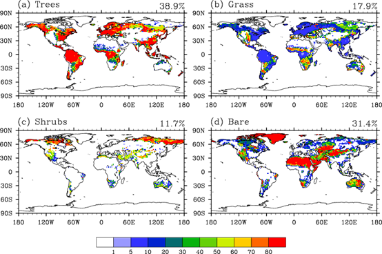
The Dynamic Global Vegetation Model (DGVM) describes the vegetation–land–atmosphere interaction. It usually consists of several modules, such as biogeochemistry, the establishment and growth of individual plants, the dynamics of population formation, biogeographical constraints, as well as environmental disturbances. Currently, it is widely used in the simulation of the global distribution of vegetation (Fig. 2) and global carbon cycling, as well as the prediction of hotspots of terrestrial ecosystem succession under future climate change. It might also be further applied to sustainable development studies, e.g., the protection and improvement of the bionomic environment through afforestation activities.
Components of the IAP DGVM.
Global vegetation distribution under current climate (simulated by the DGVM): percentage coverage of (a) trees, (b) grass, (c) shrubs and (d) bare soil.
IAP Aerosol and Atmospheric Chemical Transport Model (IAP-AACM)
Developed at IAP, CAS, IAP-AACM is the first global multi-scale nested atmospheric chemical transport model of China. It can predict the temporal and spatial variation of environment- and climate-related atmospheric chemical compositions, including trace gases (e.g. ozone, nitrogen oxides, carbon monoxide, volatile organic compounds) and aerosols (e.g. dust, sea salt, sulfate, nitrate, ammonium, black carbon, organic carbon), with a horizontal resolution of 10–300 km. The main features of IAP-AACM include: (1) its high resolution; (2) nesting from global to regional and urban scale; (3) coupled mercury chemistry and deposition module; and (4) its coupled tracer-tagging module. Applications of IAP-AACM include: (1) studying atmospheric environmental pollution (e.g. dust storms, ozone, acid rain, haze, deposition of heavy metals); (2) studying climate change (e.g. impacts of human activity, aerosol–cloud–radiation interaction, climate–emissions–air quality interaction); (3) studies for policy support (e.g. air pollution prediction and early warning, evaluation of air pollution control measures, air quality standards planning, climate change and air pollution interaction). IAP-AACM is not only a scientific research tool for the atmospheric environment and climate change, but can also be used to support environmental policymaking and guidance for daily travel.
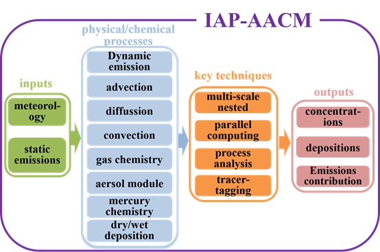
Framework of IAP-AACM.
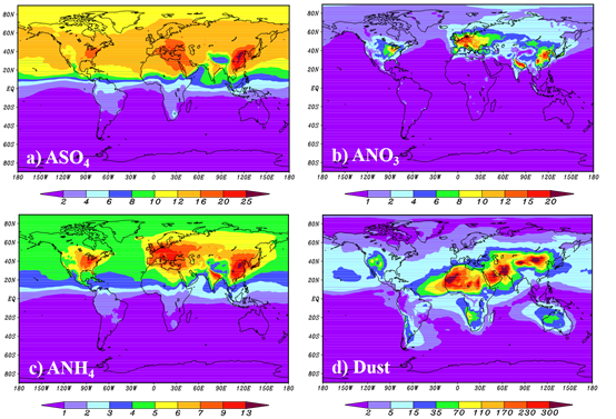
Annual mean surface concentrations (μg m−3) of atmospheric aerosol chemical compositions simulated by IAP-AACM: (a) sulfate; (b) nitrate; (c) ammonium; (d) dust.
Ocean Biogeochemical Model
The Ocean Biogeochemical Model, including two component parts of the ocean (simple biogeochemical model and ocean ecosystem model), mainly describes the biogeochemical processes of carbon in the ocean. The simple biogeochemical model describes in detail many oceanic carbon processes, such as its uptake, transformation and storage, from the exchange of CO2 at the interface between the atmosphere and the ocean. Through the simulated responses of these processes to climate change, the oceanic carbon reservoir in the mediation of the atmospheric CO2 concentration is quantified. The ocean ecosystem model mainly depicts the dynamics of plankton in the upper ocean, and provides a description of the processes for the transformation of inorganic carbon to organic carbon in terms of explicit simulations of the growth and death of plankton.
The ocean biogeochemical model provides the air–sea exchange flux of CO2 for the atmospheric circulation model to calculate the evolution of atmospheric CO2 concentrations. The ocean biogeochemical model, when fully coupled to other component models (the ESM), can be used to investigate the interaction between the carbon cycle and climate change, and to project the evolution of the ocean environment, such as pH, in the future.
Land Biogeochemical Model
The Land Biogeochemical Model can not only simulate the biogeochemical processes in the soil based on the soil environmental variables derived from the land surface model, but also provide the lower boundary of greenhouse gases for the global climate model, including CO2, methane and nitrous oxide. The establishment of this model is essential for understanding the interactions between terrestrial ecosystems and the atmosphere. The biogeochemical model is developed from the carbon or nitrogen models of Agro-C, CH4MOD and DNDC, including the processes of carbon and nitrogen transformation (decomposition, nitrification, denitrification, fermentation, etc.), transportation and related gas emissions (CO2, methane and nitrous oxide). Agro-C is a biogeophysical model for simulating regional carbon budgets of agro-ecosystems on a large scale. CH4MOD is a biogeophysical model that was developed to describe the processes of methane production, oxidation and emissions from natural freshwater wetlands and rice paddies. DNDC is a biogeochemical model for simulating the nitrogenous gas emissions from agricultural systems. The biogeochemical model will realize its target functions in the ESM via improvement to scientific processes, re-parameterization and incorporation with the land surface model at the code level.
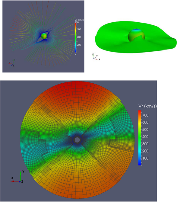
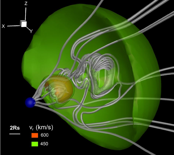
Solar–Terrestrial Space Environment Model
The Solar–Terrestrial Space Environment Model is an integration of a kinetic model and a three-dimensional magnetohydrodynamics model. Driven by solar atmosphere observations, and considering physical mechanisms like volume heating, it simulates the evolution of the solar wind from the Sun to our Earth. It can be used to study a variety of scientific issues, such as solar wind evolution characteristics during different phases of the solar activity cycle, the propagation and evolution of large-scale solar wind disturbances, and the small- and mid-scale physical processes of multi corona mass ejections/interplanetary shock interaction. The solar–terrestrial space environment model outputs the temporal and spatial variation of basic plasma and magnetic field parameters of the solar wind in near-Earth space, including velocity, mass density, energy density and strengths of each magnetic field component. The outputs can not only compensate for the scarcity of solar–terrestrial observations, but can also be utilized to analyze the interplanetary evolution of solar wind and carry out space weather forecast experiments.
Ice Sheet Model
The Ice Sheet Model is a numerical simulation system that solves equations governed by ice dynamics using the finite element method. It is capable of producing realistic simulations of ice sheet flow at the continental scale based on satellite data and results from the atmosphere and ocean models. The program will use three-dimensional full-Stokes formulation to describe the behavior of ice under gravity and internal friction, which is an advanced technique compared with most other ice shelf/sheet models (Glimmer, PISM, etc.). In addition to predicting the evolution of ice sheets under the influence of climate change, it can also be used for exploring the feedback of ice sheets to regional and global climate, as well as their effects on the global gravity and crustal stress fields.
Solid Earth Model
The Solid Earth Model is a multi-scale and multi-field system. Among the various spheres of the solid earth, the mantle convection and plate motion module deals with long-term evolution issues of the upper and lower mantle and the lithosphere; the global viscoelastic module is used to solve medium to long-term lower crustal deformation problems; the global elastic module is used to solve short-term middle-upper crustal deformation issues; the sea-storm tide and tsunami module corresponds to the hydrosphere directly influenced by earthquakes; and the landscape evolution module and regional porous elastic module are used to simulate surficial geological processes. Moreover, scientific problems associated with the solid earth always involve multi-scale module coupling. For example, the simulation of large-scale tectonic evolution needs to consider the influences of the driving force from deep mantle convection, and of the surface denudation and sedimentation.
Coupler
The coupler in CAS ESM basically originates from CPL7 in CESM. As the control center, the coupler takes charge of the communication and evolution of the various components of the ESM. It is mainly based on Model Coupling Toolkit (MCT), but with the basic data structure and algorithm of MCT having been revised and extended to support the heterogeneous supercomputing , the coupler contains many modules, such as: the time-controlling module; the computation of sensible heat, latent heat, shortwave radiation, longwave radiation, carbon flux, and fresh water modules; the two-dimensional and three-dimensional interpolation modules; the runoff interpolation module; the wind stress module; the climatological statistics module; the I/O module; the namelist and parameter files; the restart control module; the parallel and concurrent control module; and the remapping between the component models.
It also has many other significant changes compared to CESM CPL7. For instance, it introduces a registry to define and manage the coupling state and flux fields and the coupler I/O. It assembles new component models automatically by standardizing the coupling framework and through use of code-generation technology, which gets rid of time-consuming coding effort, reduces the cost, and improves the quality. It provides three-dimensional coupling algorithms and interfaces through which the regional component models will be embedded into the global component models. It expands the application of CAS ESM into the high-resolution spatial scale, the short-term temporal scale, and the regional environment manifold. In particular, it will fulfill the highly concurrent across the three tiers in CAS-ESM: the component models, the dynamical core and physical processes, and the parameterization schemes, so as to improves the parallel efficiency and maximizes the resource utilization on the supercomputing machine.